Source code: https://github.com/wrifro/wrifro.github.io/blob/main/posts/Blog_4/LinearRegression.py

Introduction & Background

Unlike Perceptron and Logistic Regression, which classify a data point (predict a specific label for it), Linear Regression is a prediction algorithm. Given features for a data point, it will predict a value for that point. The range of values Linear Regression can predict are continuous, not a finite set of labels.

The gradient is given by the formula \(\hat{w} = (X^\top X)^{-1}{X^\top}y\), but it can also be calculated using gradient descent.

As the name suggests, Linear Regression creates a linear model for a dataset, which may limit it in some settings. However, for many datasets it remains a useful prediction tool. ___

Initial Tests

As a first experiment, let’s just vizualize how the Linear Regression algorithm works.

We can begin by genarating a test dataset and a validation dataset using code from the assignment specification.

import numpy as np
from matplotlib import pyplot as plt

def pad(X):
    return np.append(X, np.ones((X.shape[0], 1)), 1)

def LR_data(n_train = 100, n_val = 100, p_features = 1, noise = .1, w = None):
    if w is None: 
        w = np.random.rand(p_features + 1) + .2
    
    X_train = np.random.rand(n_train, p_features)
    y_train = pad(X_train)@w + noise*np.random.randn(n_train)

    X_val = np.random.rand(n_val, p_features)
    y_val = pad(X_val)@w + noise*np.random.randn(n_val)
    
    return X_train, y_train, X_val, y_val

n_train = 100
n_val = 100
p_features = 1
noise = 0.2

# create some data
X_train, y_train, X_val, y_val = LR_data(n_train, n_val, p_features, noise)

# plot it
fig, axarr = plt.subplots(1, 2, sharex = True, sharey = True)
axarr[0].scatter(X_train, y_train)
axarr[1].scatter(X_val, y_val)
labs = axarr[0].set(title = "Training", xlabel = "x", ylabel = "y")
labs = axarr[1].set(title = "Validation", xlabel = "x")
plt.tight_layout()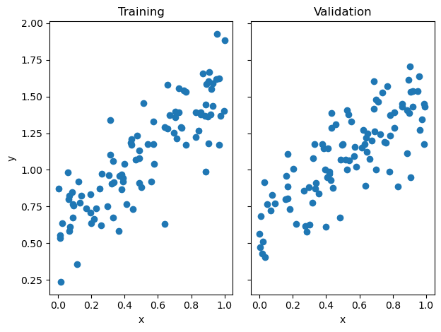

First, let’s use the analytical formula to calculate the weight vector:

from LinearRegression import LinearRegression

LR = LinearRegression()
LR.fit(X_train, y_train) # I used the analytical formula as my default fit method

LR.w

array([0.95700523, 0.60644682])

Let’s see how the training score and validation scores stack up:

I’m going to define a pad(X) function below which will allow us to add an extra feature to our test and validation data so that we can calculate the score, which allows us to vizualize the function.

def pad(X):
        return np.append(X, np.ones((X.shape[0], 1)), 1)
    
X_train_pad = pad(X_train)
X_val_pad = pad(X_val)

print(f"Training score = {LR.score(X_train_pad, y_train)}")
print(f"Validation score = {LR.score(X_val_pad, y_val)}")

Training score = 0.7134971567477733
Validation score = 0.6089993111855626

They’re quite close, indicating that this model is not overfit. ___ #### Now let’s consider the gradient descent approach:

LR2 = LinearRegression()
LR2.fit_gradient(X_train,y_train,0.001,100)

print(f"Training score = {LR2.score(X_train_pad, y_train)}")
print(f"Validation score = {LR2.score(X_val_pad, y_val)}")

Training score = 0.7040916518182994
Validation score = 0.6211301250957726

And we see that with only 100 iterations we get quite close to the same scores. Accuracy would be even greater with more iterations.

For one final test, let’s use stochastic gradient descent, which breaks the dataset into multiple batches at each step:

LR3 = LinearRegression()
LR3.fit_stochastic(X = X_train,y = y_train,alpha = 0.001,m_epochs = 100,batch_size = 10)

print(f"Training score = {LR3.score(X_train_pad, y_train)}")
print(f"Validation score = {LR3.score(X_val_pad, y_val)}")

Training score = 0.7134971567477719
Validation score = 0.6089993196979653

Training score for stochastic gradient descent is slightly higher than regular the training score for regular gradient descent but the validation score is somewhat lower. The small batches may enable the training score to rise faster; we can vizualize this later on.

Let’s vizualize this function:

w = LR.w

score_train = LR.score(X_train_pad,y_train)
score_val = LR.score(X_val_pad,y_val)

fig, axarr = plt.subplots(1, 2,constrained_layout = True)


axarr[0].scatter(X_train, y = y_train)
axarr[0].set(xlabel = "Feature 1", ylabel = "Feature 2", title = f"Training Score = {LR.score(X_train_pad, y_train)}")

f1 = np.linspace(0, 1, 101)

p = axarr[0].plot(f1, w[1] + f1*w[0], color = "black")

axarr[1].scatter(X_val, y_val)
axarr[1].set(xlabel = "Feature 1", ylabel = "Feature 2", title = f"Val Score = {LR.score(X_val_pad, y_val)}")
p2 = axarr[1].plot(f1, w[1] + f1 * w[0], color = "black")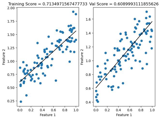

This is more or less what you would expect! A line that does not perfectly predict any point, but instead seems to be somewhere in the middle of all the points. ___ ### Experiments

Let’s plot the score history over 100 iterations of standard gradient descent versus stochastic gradient descent to see which achieves a higher training score faster:

plt.plot(LR2.score_history)
plt.plot(LR3.score_history)
labels = plt.gca().set(xlabel = "Iteration", ylabel = "Score")
title = plt.gca().set(title = f"Score = {LR2.score(X_train_pad, y_train)}")
ylim = plt.gca().set_ylim([-0.5, 1])
legend = plt.gca().legend(["Regular Gradient Descent","Stochastic Gradient Descent"])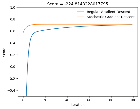

Interesting. It is quite clear that stochastic gradient descent very rapidly achieves a highly accurate training score, while the standard gradient descent algorithm takes longer to reach the same point.

Now let’s consider what happens as the number of features approaches the number of training points…

We can accomplish this by running our algorithm on a dataset with 100 points 100 different times, with the number of features increasing from 1-99 with each iteration.

Then, let’s plot the training score vs validation score to see how they compare.

n_train = 100
n_val = 100
p_features = 1
noise = 0.2
w = None

training_scores = []
val_scores = []

for i in range (1,100):
    p_features = i
    X_train, y_train, X_val, y_val = LR_data(n_train, n_val, p_features, noise)
    LRtemp = LinearRegression()
    LRtemp.fit(X_train,y_train)
    train_score = LRtemp.score(pad(X_train),y_train)
    val_score = LRtemp.score(pad(X_val),y_val)
    training_scores.append(train_score)
    val_scores.append(val_score)

plt.plot(val_scores)
plt.plot(training_scores)
ylim = plt.gca().set_ylim([0, 1.5])
title = plt.gca().set(title = f"Training score = {training_scores[-1]}, Val score = {val_scores[-1]}")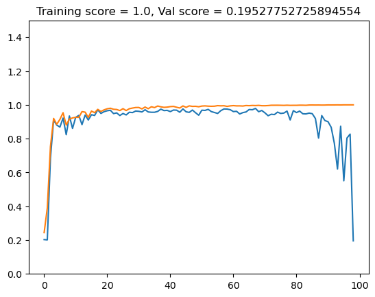

Fascinating! Training score has risen to a perfect 1.0, while the validation score closely tracked it for a while before dropping off rapidly as number of features rose.

This seems to be a perfect example of “overfitting”. Faced with a complicated dataset, the model generates a solution that perfectly fits the complex testing data but is useless when faced with other data.

Lasso Regularization

We can replicate a similar experiment using the LASSO model instead of linear regression. Lasso should in theory stabilize some of the large differences between the validation and testing scores.

from sklearn.linear_model import Lasso

lasso_train = []
lasso_val = []

for i in range (1,100):
    p_features = i
    X_train, y_train, X_val, y_val = LR_data(n_train, n_val, p_features, noise)
    L = Lasso(alpha = 0.001)
    L.fit(X_train,y_train)
    train_score = L.score(X_train,y_train)
    val_score = L.score(X_val,y_val)
    lasso_train.append(train_score)
    lasso_val.append(val_score)

plt.plot(lasso_val)
plt.plot(lasso_train)
title = plt.gca().set(title = f"Training score = {lasso_train[-1]}, Val score = {lasso_val[-1]}")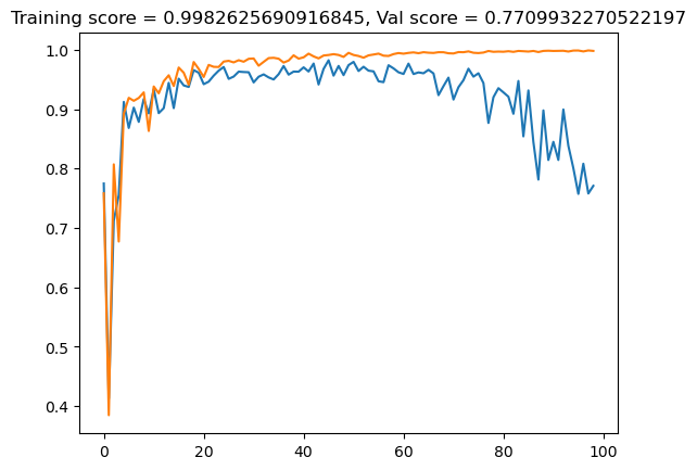

The validation score is better than for the linear regression model, but still dropps off towards the end, indicating overfitting.

What happens if we increase alpha by a factor of ten?

lasso_train1 = []
lasso_val1 = []

for i in range (1,100):
    p_features = i
    X_train, y_train, X_val, y_val = LR_data(n_train, n_val, p_features, noise)
    L = Lasso(alpha = 0.01)
    L.fit(X_train,y_train)
    train_score = L.score(X_train,y_train)
    val_score = L.score(X_val,y_val)
    lasso_train1.append(train_score)
    lasso_val1.append(val_score)

plt.plot(lasso_val1)
plt.plot(lasso_train1)
title = plt.gca().set(title = f"Training score = {lasso_train1[-1]}, Val score = {lasso_val1[-1]}")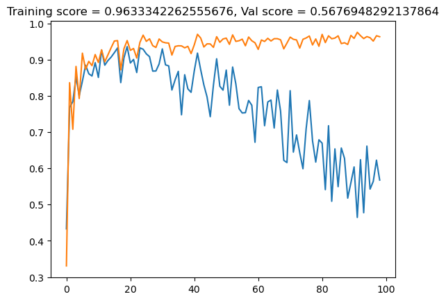

As alpha, which in the case of lasso controls the strength of the regularization, increases by a factor of ten to 0.1, the validation and testing scores differ even more than when alpha was 0.001.

And what if we increase once more by a factor of ten?

lasso_train2 = []
lasso_val2 = []

for i in range (1,100):
    p_features = i
    X_train, y_train, X_val, y_val = LR_data(n_train, n_val, p_features, noise)
    L = Lasso(alpha = 0.1)
    L.fit(X_train,y_train)
    train_score = L.score(X_train,y_train)
    val_score = L.score(X_val,y_val)
    lasso_train2.append(train_score)
    lasso_val2.append(val_score)

plt.plot(lasso_val2)
plt.plot(lasso_train2)
title = plt.gca().set(title = f"Training score = {lasso_train2[-1]}, Val score = {lasso_val2[-1]}")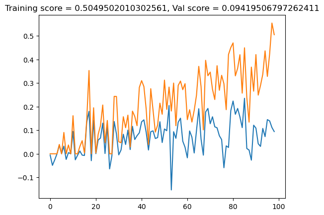

This seems to basically break the whole algorithm.

So, it is clear that under certain circumstances – namely, when number of features approaches the number of data points – the LASSO model may be a better approach than linear regression. But it is not a magic bullet, and as the tests above show, it is difficult to find the correct formula to keep training and validation scores close.

Conclusion

The power of the linear regression model is apparent from these tests. Rather than focusing on labeling datapoints, it is able to come up with a model that predicts what a hypothetical datapoint’s value should be based on the values of the other datapoints. There are slight differences between the different approaches to the model - stochastic gradient descent achieves an optimal result with impressive speed, for example - but at the end of the day all of the different approaches yield more or less the same result.